


| Derivatives | |
| diff(ex,t) | the derivative of an expression with respect to t |
| function_diff(f) | the derivative of a function |
| diff(ex,x$n,y$m) | partial derivatives |
| grad | gradient |
| divergence | divergence |
| curl | curl |
| laplacian | laplacian |
| hessian | hessian matrix |
The diff function will find the derivative of an expression and returns the derivative as an expression. If you have a function f, you can find the derivative by entering
diff(f(x),x)
Note that the result will itself be an expression; do not define the deritivave function by fprime(x) := diff(f(x),x). If you want to define the derivative as a function, you can use unapply:
fprime := unapply(diff(f(x),x),x)
Alternatively, you can use function_diff, which takes a function (not an expression) as input and returns the derivative function;
fprime := function_diff(f)
The diff function can take a sequence of variables as the second argument, and so can calculate successive partial derivatives. Given
E := sin(x*y)
then
diff(E,x)
will return
| y*cos(x*y) |
diff(E,y)
will return
| x*cos(x*y) |
diff(E,x,y)
will return
| −x*y*sin(x*y) + cos(x*y) |
and
diff(E,x $ 2)
will return
| −y2*sin(x*y) |
If the second argument to diff is a list, then a list of derivatives is returned. For example, to find the gradient of E, you can enter
diff(E,[x,y])
and get
| [y*cos(x*y),x*cos(x*y)] |
There is also a special grad command for this, as well as commands for other types of special derivatives.
| Limits and series | |
| limit | the limit of an expression |
| taylor | Taylor series |
| series | Taylor series |
| order_size | used in the remainder term of a series expansion |
The limit function will take an expression, a variable and a point and return the limit at the point. If you enter
limit(sin(x)/x,x,0)
you will get
| 1 |
Xcas can also find limits at plus and minus infinity;
limit(sin(x)/x,x,+infinity)
will return
| 0 |
as well as limits of infinity;
limit(1/x,x,0)
will return
| ∞ |
which recall is unsigned infinity. An optional fourth argument can be used to find one-sided limits; if the fourth argument is 1 it will be a right-handed limit and if the argument is -1 it will be a left-handed limit. Entering
limit(1/x,x,0,-1)
will result in
| −∞ |
Given an expression and a variable, the taylor function will find the Taylor series of the expression. If you enter
taylor(sin(x)/x,x)
you will get
| 1− |
| + |
| + x6*order_size(x) |
The series function works the same as the taylor function.
By default, taylor will find the terms up to the fifth degree. The order_size(x) represents a factor for which for all a>0, the term xaorder_size(x) will approach 0 as x approaches 0.
The series returned by taylor will also be centered about 0 by default; if you want to center it around the number a, you can replace x by x=a;
taylor(exp(x),x=1)
will result in
| exp(1)+exp(1)*(x−1)+exp(1)*(x−1)2/2+ exp(1)*(x−1)3/6+ |
| exp(1)*(x−1)4/24+exp(1)*(x−1)5/120+(x−1)6*order_size(x−1) |
You can also give the center of the series with a third argument. To find the terms to a different you can add an extra argument giving the order;
taylor(sin(x)/x,x=0,3)
will return
| 1− |
| + x4*order_size(x) |
Note that in this case you must explicitly give the center of the series, even if it is 0.
To find the Taylor polynomial, you can add an extra argument of polynom;
taylor(sin(x)/x,x,polynom)
will return
| 1− |
| + |
|
| Integrals | |
| int | antiderivatives and exact integrals |
| romberg | approximation of integrals |
The int function will find an antiderivative of an expression. By default, it will assume that the variable is x, to use another variable you can give it as an argument.
int(x*sin(x))
will result in
| sin(x) − x*cos(x) |
and
int(t*sin(t),t)
will result in
| sin(t) − t*cos(t) |
To compute a definite integral, you can give the limits of integration as arguments after the variable; to integrate x*sin(x) from x=0 to x=π, you can enter
int(x*sin(x),x,0,pi)
and get
| π |
The limits of integration are allowed to be expressions; this can be useful when computing a multiple integral over a non-rectangular region. For example, you can integrate x y over the triangle 0 ≤ x ≤ 1, 0 ≤ y ≤ x with
int(int(x*y,y,0,x),x,0,1)
resulting in
|
The romberg function will approximate the value of a definite integral, for cases when the exact value can’t be computed or you don’t want to compute it. For example,
romberg(exp(-x^2),x,0,10)
will return
| 0.886226925452 |
| Solving equations | |
| solve(eq,x) | exact solutions of an equation |
| solve([eq1,eq2],[x,y]) | exact solutions of a system of equations |
| fsolve(eq,x) | approximate solution of an equation |
| fsolve([eq1,eq2],[x,y]) | approximate solution of a system of equations |
| linsolve | solve a linear system |
| proot | approximate roots of a polynomial |
Solving equations is important, but it is often impossible to find exact solutions. Xcas has the ability to find exact solutions in some cases and to approximate solutions.
The solve function will attempt to find the exact solution of an equation that you give it. If you enter an expression that isn’t an equation, it will try to solve for the expression equal to zero. By default, the variable will be x, but you can give a different variable as a second argument. If you enter
solve(x^3 -2*x^2 + 1=0, x)
you will get
| ⎡ ⎢ ⎢ ⎣ |
| ,1, |
| ⎤ ⎥ ⎥ ⎦ |
By default, solve will only try to find real solutions; if you enter
solve(x^3+1=0,x)
you will get
| [−1] |
You can configure Xcas to find complex solutions (see section 2.3, “Configuration”). If you do that, then entering
solve(x^3+1=0,x)
will result in
| ⎡ ⎢ ⎢ ⎣ | −1, |
| , |
| ⎤ ⎥ ⎥ ⎦ |
For linear and quadratic functions, solve will always return the exact solution. For higher degree polynomials, solve will try some approaches, but may return intermediate results or approximate solutions. (It doesn’t use the Cardan and Ferrari formulas for polynomials of degrees 3 and 4, since the solutions would then not be easily managable.)
For trigonometric equations, the primary solutions are returned. For example,
solve(cos(x) + sin(x) = 0, x)
will result in
| ⎡ ⎢ ⎢ ⎣ | − |
| , |
| ⎤ ⎥ ⎥ ⎦ |
You can configure Xcas to find all solutions (see section 2.3, “Configuration”). If you do that, then
solve(cos(x) + sin(x) = 0, x)
will result in
| ⎡ ⎢ ⎢ ⎣ |
| ⎤ ⎥ ⎥ ⎦ |
where n0 represents an arbitrary integer.
The solve function can also handle systems of equations. For this, use a list of equations for the first argument and a list of variables for the second. If you enter
solve([x^2 + y - 2, x + y^2 - 2],[x,y])
you will get all four solutions as a matrix; each row represents one solution.
| ⎡ ⎢ ⎢ ⎢ ⎢ ⎢ ⎢ ⎢ ⎢ ⎢ ⎢ ⎢ ⎢ ⎢ ⎢ ⎢ ⎣ |
| ⎤ ⎥ ⎥ ⎥ ⎥ ⎥ ⎥ ⎥ ⎥ ⎥ ⎥ ⎥ ⎥ ⎥ ⎥ ⎥ ⎦ |
To approximate a solution to an equation or system of equations, Xcas provides the fsolve command. If you enter
fsolve(x^3 -3*x + 1,x)
you will get
| [−1.87938524157,0.347296355334,1.53208888624] |
Algorithms for approximating solutions of equations typically involve starting with a given point and finding a sequence which converges to a solution. The fsolve command can take a starting point, if you enter
fsolve(x^3 -3*x + 1,x,1)
you will get
| 0.347296355334 |
| Commands for differential equations | |
| desolve | exact solution |
| odesolve | approximate solution |
| plotode | graph of solution |
| plotfield | vector field |
| interactive_plotode | clickable interface |
The desolve command is used to try to find exact solutions of differential equations. The first argument is the differential equation itself, the second argument is the function. The derivative of an unknown function y is denoted diff(y), which can be abbreviated y’. The second derivative will be diff(diff(y)) or y’’, etc. If you enter
desolve(x^2*y’ = y,y)
you will get
| c0 * exp(− |
| ) |
where c0 is an arbitrary constant. By default the variable is x, if you want to use a different variable, put it in the function in the second argument;
desolve(t^2*y’ = y,y(t))
will return
| c0 * exp(− |
| ) |
If you want to solve a differential equation with initial conditions, the first argument should be a list with the differential equation and the conditions. If you enter
desolve([y’’ + 2*y’ + y = 0, y(0) = 1, y’(0) = 2],y)
you will get
| exp(−x)*(3*x+1) |
To solve a differential equation numerically, you can use the odesolve command. This will allow you to solve the equation y′=f(x,y) where the graph passes through a point (x0,y0). The command
odesolve(f(x,y),[x,y],[x_0,y_0],a)
will find y(a) in this case. For example, to calculate y(2) where y(x) is the solution of y′(x) =sin(xy) with y(0)=1, you can enter
odesolve(sin(x*y),[x,y],[0,1],2)
The result will be
| [1.82241255674] |
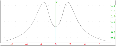
The plotode command will plot the graph of the solution; if you enter
plotode(sin(x*y),[x,y],[0,1])
you will get
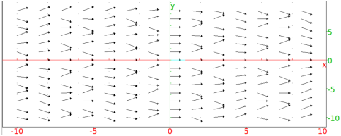
The plotfield command will plot the entire vector field;
plotfield(sin(x*y),[x,y])
will result in
If you use the interactive_odeplot command, you will get the vector field and you will be able to click on a point to find the graph of the solution passing through the point.