$\chi$ CAS for the TI84

Bernard.Parisse@univ-grenoble-alpes.fr

2024

Abstract: This document explains how to run $\chi$ CAS, an (extra)-light version of the Giac/Xcas computer algebra system (CAS) for the TI84 calculator. The app is like a second calculator, a CAS calculator, inside your TI84.

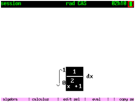
A few screenshots to illustrate that $\chi$ CAS is not just a CAS, but really a second calculator : the shell, input of a 2d expression, result of another calculation displayed in 2d,

graph of a function (with 60% more pixels), speed and normal pointing to the center of the osculating circle, a parametric curve

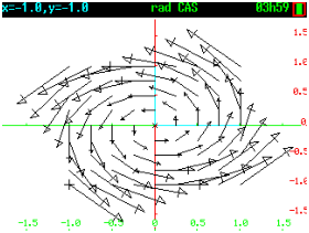
vector field plot

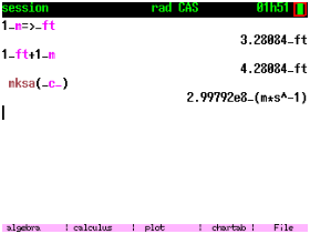
unit conversion and computation

This document is interactive, you can modify and run commands by clicking in the ok button or by hitting Enter.

1 Introduction

The first time porting Xcas to the 84 was reported on the tiplanet forum, it was an April fool. It seemed indeed almost impossible to do on this ez80 CPU, an evolution of the z80 created about 50 years ago. TI itself choosed a 68000 processor for the TI92/voyage 200 CAS and later an arm32 processor for the ti nspire family and they recently choosed to add a coprocessor to the 84 in order to run MicroPython. But the expert users community of the ti84 did a wonderful job, using and creating free software, with a huge work of reverse engeneering, they made it possible to port KhiCAS. It required several months of development on my side, but it is now a reality: KhiCAS is available on the ti84.

There is however a price to pay: I had to remove a lot of functionnalities compared to other KhiCAS ports. I tried to keep the essential features, that should be sufficient for highschool students and probably also later. The CPU speed is also slow compared to calculator of other manufacturers, be prepared to wait a few seconds for every non trivial computation, and sometimes more. But the execution environment is safer than with other calculators: you can easily archive sessions and programs, and a simple reset will not loose any data on recent OSes.

2 Installation

KhiCAS installation is not a straightforward install like other apps because it is not a TI app. [Legal stuff] Beware: the install process was checked several times, but I can not warrant that everything will work without issues on your calculator, therefore the author declines all responsability. [End of legal stuff].
Please follow carefully the install process below. First of all check your current OS version (2nd mem 1). If your calculator freezes during the install process, don’t panic. It is possible to restore factory defaults by pressing 2nd and del and reset the calc while keeping 2nd and del pressed, then release 2nd and del, press cancel and send the same OS version again. Check that it is exactly the same version of your OS, smaller versions will not install, and if you install a higher version, you will not be able to downgrade anymore, which means more restrictions (e.g. running ASM programs will become more complicated), and might render KhiCAS incompatible with your calculator. Do not install OS from TI website before checking that it remains compatible with KhiCAS. After discussions with TI, it has been agreed that KhiCAS would not run on the latest OS version.

KhiCAS install process

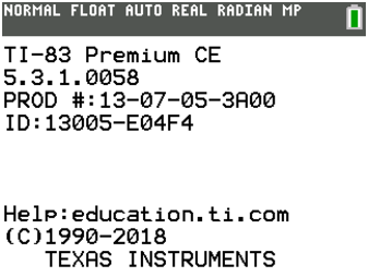
Before beginning, check which OS version is installed on your calc with 2nd mem 1, on the following screen capture it is 5.3.1

Download the very same OS version from tiplanet, in case there is a problem during install and you would have to reflash the calculator OS after 2nd-del-reset cancel.
Now get $\chi$ CAS for TI84.
The current install process requires that you purge the archive memory of your calculator, including language packages. Therefore backup your data and applications and lang packs with TI Connect CE.
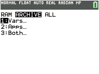
Then 2nd mem 7 rightarrow 3 2
Send INST, artifice and all the files of the app folder to the calculator, in order.
Alternative, only valid for Windows users: send khicas84.b84 to the calc.
Alternative with TILP under Unix : run the script transfert_tilp.sh (don’t use the GUI, it would send the files in reversed order).
Note that the install process below will clear remaining apps and language packs.
If you have OS version strictly smaller than 5.5, you can run INST from prgm key and skip the rest of this item.
If you have OS version 5.5 or greater, you must first enable ASM. Procedure: send CabriJr, open Cabri from app, type enter then F1 then down to Open, and open artifice (from YvanTT). This will “jailbreak” the calculator, restoring ASM. Now select INST
Important : the calc will reboot after INST is finished, but this is not enough, you must clear the RAM with 2nd mem 7 1 2 before calling KhiCAS (app key)
You can now remove remaining install AppVars (2nd mem 2 alpha B) and restore your lang pack if it’s not English. This should leave you with 128K to 256K of archive (depending on the final configuration).

Beware

After discussions with TI, it has been agreed that KhiCAS would not run on the latest OS version.
Do not upgrade your calculator OS from TI site. If you want to upgrade your calculator OS, get a version from tiplanet after you have checked that it remains compatible with $\chi$ CAS on tiplanet or on cemetech.
CAS is not allowed at some exams in some countries. It is your responsability to check if CAS calculators are allowed before running $\chi$ CAS in a test. The authors decline all responsabilities for any misuse.
For example, as of 2024 November 16th, CAS are allowed at SAT tests, but CAS are not allowed at ACT tests.
Therefore you can have KhiCAS installed on your TI84 for SAT (note that the CAS feature is not included in Desmos calculator, it is only available on CAS calculators like TI Nspire CXII CAS or HP prime and KhiCAS compatible calculators like TI84, Casio fxcg50 and Numworks). But don’t forget to remove it from your TI84 for ACT.

3 First steps

Type app and 2 to run KhiCAS. This opens the “shell” (or history) where you can write Xcas commands. The math key will open a menu of important CAS commands, the most commonly CAS commands may be retrieved with fast menus obtained by pressing the 5 keys below the screen, these keys may be prefixed with 2nd or alpha, according to the legend at the bottom. The application menu (save/restore sessions, ...) is assigned to the graph key (alpha label F5).

For example, type 1/2+1/6 then enter, you should see the result 2/3 displayed below.

Hint : If you can not find a character on the calculator keyboard, press trace (chartab).

You can copy a level from the history of commands by hitting the up and down arrow keys (once or more) and enter. Then you can modify the command and run it with enter. For example, up arrow twice, enter, replace 1/6 by 1/3 and hit enter. Another example as a screenshot

If the result of your command is an expression, like x+1, it will be displayed in the 2d expression editor. Type cancel to leave the expression editor.

It is recommended to store the result in a variable if you want to reuse it later. There are two ways to store a value in a variable

right-store with => using the sto key for example 2=>a stores 2 in variable a. Now, every time you write a in a computation, it will be replaced by 2.
left-store with :=. Since it requires many keystrokes, = (2 keystrokes: window 8 or sto del) is accepted as a synonym for most simple commands.

Type the var key to display the current variables assigned. This will also display the total amount of contiguous RAM available for computations. If this value is near 0, you should leave KhiCAS and enter it again (this will garbage collect the RAM available for CAS computations).

The most popular Xcas commands are available from fast menus shortcuts : Y= (F1, algebra), window (F2, calculus) and 2nd-F1 to F5 or alpha F1 to F5 short menus, or from the math key menu, where there is a short online help with an example for each command.
Example 1 : type the window key, move to the desired item then enter or type it’s number

Example 2 : hit math, choose a submenu, e.g. Algebra, hit enter, move the selection to a command, for example factor. Now type graph (F5) to display a short help with an example. Hit F2 or F3 to copy the example in the commandline. You can run the example as is (enter) or modify it and run it (enter) if you want to factor another polynomial. If you have already entered the command in the commandline, type the down cursor key or the key on the row above $x^2$ to open the catalog at this command and F5 to get help (if available, unfortunately there is not enough room to store help for all commands).

If you prefer entering an expression in 2-d mode, type 2nd X,T,... For example, enter $\frac{\sin(x)}{x}$ like this: 2nd X,T,.., this will display 0 selected, type x enter, this will replace the selection by $x$ , type the sin key, this will apply sin on the selection and display $\sin(x)$ selected, type the division key, this will display $\frac{\sin(x)}{0}$ with 0 selected, type x enter and you get $\frac{\sin(x)}{x}$ . Type enter when you are finished, this will copy the expression in the commandline. Another example in screenshots :

The KhiCAS File menu (F5) has an item Clear that will erase the history. This will not clear the variables, to achieve that type the var, select the last item restart and confirm with enter.

Hit 2nd quit to leave $\chi$ CAS. Variables and history are saved each time you run a command with enter, they will be restored if you come back to $\chi$ CAS.

4 Common CAS commands

4.1 Expand and factor

From math commands catalog, select Algebra, or type 2nd-1.

factor : factorization. Shortcut =>* (sto key then *), for example
x^4-1=>*
. Run cfactor to factor over $\C$ .
partfrac : expands a polynomial or performs partial fraction expansion over a fraction. Shortcut =>+ (sto then + key), for example
(x+1)^4=>+
or
1/(x^4-1)=>+
.
simplify : tries to simplify an expression. Shortcut =>/ (sto key then /), for example
sin(3x)/sin(x)=>/
ratnormal : rewrite as an irreducible fraction.

4.2 Calculus

From math commands catalog, select Calculus, or type 2nd-2

diff : derivative. Shortcut ' for derivative with respect to $x$ , example
diff(sin(x),x)
and
sin(x)'
are equivalent. For $n$ th-derivative, add $n$ , for example 3rd derivative
diff(sin(x^2),x,3)
.
integrate : antiderivative (1 or 2 or 4 arguments) for example
integrate(sin(x))
or
integrate(1/(t^4-1),t)
for $\int \frac{1}{t^4-1} \ dt$
Defined integration with 4 arguments, for example
integrate(sin(x)^4,x,0,pi)
computes $\int_0^\pi \sin(x)^4 \ dx$ . For an approximate computation, enter one boundary as an approx number, for example
integrate(sin(x)^4,x,0.0,pi)
limit : limit of an expression. Example
limit((cos(x)-1)/x^2,x=0)
taylor and series : Taylor expansion or asymptotic serie expansion, for example taylor(sin(x),x=0,5)

Add polynomial if you do not want to have the remainder term.
sum : discrete summation, for example
sum(k^2,k,1,n)
computes $\sum_{k=1}^n k^2$ ,
sum(k^2,k,1,n)=>*
computes the sum and rewrites it factored.

4.3 Solvers

From math commands catalog, select Solve.

solve solves an equation exactly. Takes the variable to solve for as second argument, unless it is x, for example
solve(t^2-1=0,t)
.
If exact solving fails, run fsolve for approx solving, either with an iterative method starting with a guess
fsolve(cos(x)=x,x=0.0)
or by dichotomy
fsolve(cos(x)=x,x=0..1)

For complex solutions, run csolve.
It is possible to restrict solutions using assumptions on the variable, for example
assume(m>1)
then
solve(m^2-4=0,m)
.
solve can also solve (simple) polynomial systems, enter a list of equations as 1st argument and a list of variables as 2nd argument, for example intersection of a circle and a line:
solve([x^2+y^2+2y=3,x+y=1],[x,y])
Run linsolve to solve linear systems. enter a list of equations as 1st argument and a list of variables as 2nd argument, example:
linsolve([x+2y=3,x-y=7],[x,y])
Run desolve to solve exactly a differential equation. for example, to solve $y'=2y$ , type desolve(y'=2y).
Another example with an initial condition:
desolve([y'=2y,y(0)=1],x,y)

4.4 Arithmetic

When required, the distinction between integer arithmetic and polynomial arithmetic is done by a prefix i for integer commands. For example ifactor for integer factorization and factor for polynomial factorization (or cfactor for polynomial factorization over $\C$ ). Some commands work for integers and polynomials, like gcd and lcm.

4.4.1 Integers

From math catalog, select Arithmetic, Crypto.

iquo(a,b), irem(a,b) quotient and remainder of euclidean division of two integers.

iquo(23,13),irem(23,13)
isprime(n) checks whether $n$ is prime. This is a probabilisitic test for large values of $n$ .
isprime(2^64+1)
ifactor(n) factorizes an integer (not too large, since algorithms used are trial division and Pollard- $\rho$ , there is not enough RAM for quadratic sieve), for example
ifactor(2^64+1)

Shortcut sto then * (=>*)
gcd(a,b), lcm(a,b) GCD and LCM of two integers or polynomials.

gcd(25,15),lcm(25,15)

gcd(x^3-1,x^2-1),lcm(x^3-1,x^2-1)
iegcd(a,b) (integer extended GCD) returns 3 integers $u,v,d$ such that $au+bv=d$ where $d$ is the GCD of $a$ et $b$ , $|u|<|b|$ and $|v|<|a|$ .

u,v,d:=iegcd(23,13); 23u+13v
ichinrem([a,m],[b,n]) returns (if possible) $c$ such that $c=a \pmod m$ and $c=b \pmod n$ (if $m$ are $n$ coprime, $c$ exists).
c,n:=ichinrem([1,23],[2,13]); irem(c,23); irem(c,13)
powmod(a,n,m) returns $a^n \pmod m$ computed by the fast modular powering algorithm

powmod(7,22,23)
asc converts a string to a list of ASCII code, char converts back a list to a string. These commands may be used to easily write cryptographic algorithms with string messages.

4.4.2 Polynomials

From math catalog, select Polynomials.

The default variable is $x$ , otherwise you can specify it as last optional argument. For example degree(x^2*y) or degree(x^2*y,x) return 2, degree(x^2*y,y) returns 1.

Polynomials may have coefficients in the rationals (example 2/3*x+1), or floats (example 0.5*x+1), or in $\mathbb{Z}/p\mathbb{Z}$ (example 3*x+5 mod 7) or in a Galois fields (example, call once GF(2,4) to define the finite field with 16 elements with generator g by default, then g^2*x+g+1)

coeff(P,n) coefficient of $x^n$ in $P$ , lcoeff(P) leading coefficient of $P$ , for example
P:=x^3+3x; coeff(P,1); lcoeff(P)
degre(P) degree of polynomial $P$ degree(x^3)
quo(P,Q), rem(P,Q) quotient and remainder of euclidean division of P by Q
P:=x^3+7x-5; Q:=x^2+x; quo(P,Q); rem(P,Q)
proot(P) : approx. roots of $P$ (all roots, real and complex)
proot(x^5+x+1)
interp(X,Y) : for two lists of the same size, returns the interpolating polynomial $P$ such that $P(X_i)=Y_i$ .

X,Y:=[0,1,2,3],[1,-3,-2,0]; P:=interp(X,Y)=>+
resultant(P,Q) : resultant of polynomials $P$ and $Q$ P:=x^3+7x-5; Q:=x^2+x; resultant(P,Q)
tchebyshev1(n) and tchebyshev2(n) Tchebyshev polynomials of 1st and 2nd kind defined by : $T_n(\cos(x))=\cos(nx), \quad U_n(\cos(x))\sin(x)=\sin((n+1)x)$

4.5 Linear algebra, vectors, matrices

Xcas does not make distinction between vectors and lists. For example,

v:=[1,2]; w:=[3,4]

onload
defines 2 vectors $v$ and $w$ , then dot will compute the scalar product of $v$ and $w$ : dot(v,w)

A matrix is a list of lists of the same size. You can enter a matrix element by element using the matrix editor (2nd-7 enter or 2nd-enter i). Enter a new variable name to create a new matrix or the name of an existing variable to edit a matrix. The , key may be used to insert a line or column, and the Del key erases the line or column of the selection. Type 2nd-3 if you want to undo one edition step. For small matrices, it is also convenient to enter them directly in the commandline, for example to define $A=\left(\begin{array}{cc} 1 & 2 \\ 3 & 4 \end{array}\right)$ type

A:=[[1,2],[3,4]]

onload
or
[[1,2],[3,4]]=>A
It is recommended to store matrices in variables!

If a matrix is defined by a formula, then it’s better to use the matrix command (2nd-7 enter Cancel), for example:
matrix(2,2,(j,k)->1/(j+k+1))
returns the matrix where coefficient line $j$ and column $k$ is $\frac{1}{j+k+1}$ (beware, indices begin at 0).

Run idn(n) to get the identity matrix of order $n$ and ranm(n,m,law,[parameter]) to get a matrix with random coefficients with dimensions $n,m$ . for example
U:=ranm(4,4,uniformd,0,1)

N:=ranm(4,4,normald,0,1)

For basic arithmetic on matrices, use keyboard operators (+ - *, inverse). Otherwise, open catalog and select Matrices

egvl(A)

egv(A)
eigenvalues and eigenvectors of matrix $A$ .
P,D:=jordan(A)
finds the Jordan normal form of matrix $A$ , returns matrices $P$ and $D$ such that $P^{-1}AP=D$ , with $D$ upper triangular (diagonal if $A$ is diagonalizable)
Ak:=matpow(A,k)
computes matrix $A$ to the $k$ -th power, where $k$ is symbolic.
rref: row reduction to echelon form
lu: $LU$ factorization of matrix $A$ , returns a permutation $P$ and two matrices $L$ (lower) and $U$ (upper) such that $PA=LU$ . The result of P,L,U:=lu(A)
may be passed as an argument to the command linsolve(P,L,U,v)
to solve a system $Ax=b$ by solving two triangular systems (in $O(n^2)$ instead of $O(n^3)$ ).

5 Spreadsheet, statistics

Type the stat key to open the spreadsheet. The spreadsheet UI can display some graphics including statistic graphics.

The spreadsheet is using usual notations, with one little exception, row indices begin at 0 (like in programming).

Shortcuts for = and $ : like with TI cellsheet, press sto or 2nd sto.

Cell edit: type any character (this will erase the previous cell content) or type [trace] 4 (edit cell item).

For cell cross-reference in a commandline, you can key in the cell name (lowercase is accepted for row index) or the cell range. Or press the up or down arrow key, then move to the cell and press enter. If you want to input a range, instead of pressing enter, press stats or [trace] 2 (fast menu for edit, select), and move to the opposite cell of the rectangular selection, and press enter. Or alternatively, type alpha :, then up or down cursor, move to the opposite cell.

Statistics on a range : move to the first cell of the data, press stats, move to the last cell in the same column or in an adjacent column and press stats again. If the selection is on 1 column, this will display 1-d stats (mean, standard deviation, min, first quartile, median, third quartile, max), if the selection is on 2 columns, this will display covariance and correlation. If you want to do further computations with these values, leave the spreadsheet (2nd quit) to the shell and type 2nd ins. If you want to have statistics that are updated each time you change the data, then move to an unused cell, type sto (to enter =) and select a stats command from stat1d/stat2d or from the catalog then the range of the data.

Copy/paste of a range : Move to a vertex of a rectangular range, type stats (or [trace] 2 for the select item of edit menu), move to the opposite vertex and type [trace] 2. The selection can be pasted with 2nd ins in the spreadsheet, or in the shell (in that case the cell values are pasted as a matrix).

If you want to have a graphic representation from data in the spreadsheet, go to a cell that is currently not used, type = (sto key), then enter a command (using the menus), then make a selection like explained above. Type 2nd stat plot to display the graph.
Example: scatterplot and linear regression plot for some data in columns 1 and 2
Enter data, move to an unused cell, type sto then window (stat2d) enter

last screenshot after move to the range begin, then type stat and move to the range end, then enter

2nd graph stat will display the points, type - to zoom out and see all the points

move to another unused cell, type window (stats2d), select item 4, enter the range (entered from keyboard in the screenshot), enter, then 2nd graph stats

Leave the spreadsheet to see the line equation and the $r^2$ coefficient.

N.B.: for probability distributions, please go back to TI OS shell, there is not enough room in user flash to provide an implementation inside KhiCAS.

6 Graphics

Inside KhiCAS, one gets a graphical representation by entering a command that returns a graphic object (see next section 6.1), then this graphic object will be displayed in the graphic application (see section 6.2). The whole display, except the status area, will be used to display the graphic object, i.e. 320 $\times$ 222 pixels instead of 265 $\times$ 165 pixels for TI OS graphical application, 62% more pixels!

6.1 Graphic commands

From math catalog, select Graphics (or type the plot fast menu shortcut [zoom]) and choose a graphic command. If you want to have more than one curve on the same graphic, enter several commands with ; as separator.

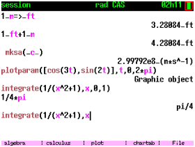
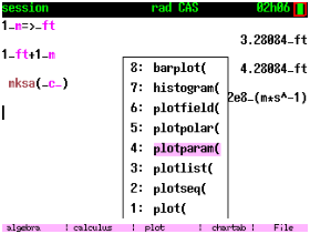
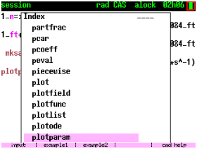
Screenshots illustrating access to a parametric plot command: first press zoom (plot fast menu), then move to plotparam enter (or type 5), then press the key above the $x^2$ key, then the graph key to get help, then F2 to copy the example.

plot(f(x),x=a..b) plot expression $f(x)$ for $x\in [a,b]$ . Discretization option: xstep=, for example plot(x^2,x=-4..4,xstep=1)
Default is 384 evaluations per plot (one per horizontal pixel).
plotseq(f(x),x=[u0,a,b]) webplot for a recurrent sequence $u_{n+1}=f(u_n)$ of first term $u_0$ , for example if $u_{n+1}=\sqrt{2+u_n}, u_0=6$ , with a plot on $[0,7]$ plotseq(sqrt(2+x),x=[6,0,7])
plotparam([x(t),y(t)],t=tm..tM) parametric plot $(x(t),y(t))$ for $t\in [t_m,t_M]$ . Discretization option: tstep=. Example plotparam([sin(2t),cos(3t)],t,0,2*pi)
plotpolar(r(theta),theta=a..b) polar plot of $r(\theta)$ for $\theta \in [a,b]$ , for example plotpolar(sin(3*theta),theta,0,2*pi)
plotlist(l): plot a list l, i.e. draws a polygonal line with vertices $(i,l_i)$ (index $i$ starts at 0).
plotlist([X1,Y1],[X2,Y2],...) polygonal line with vertices the points of coordinates $(X_i,Y_i)$
scatterplot(X,Y), polygonscatterplot(X,Y) for two lists X,Y of the same size, draws the points or a polygonal line of vertices $(X_i,Y_i)$
histogram(l,class_min,class_size) plots the histogram of data in l, class size class_size, first class starts at class_min. Example: check the random generator quality
l:=ranv(500,normald,0,1); histogram(l,-4,0.25); plot(normald(x),x,-4,4)
plotfield(f(t,y),[t=tmin..tmax,y=ymin..ymax]) plot the field of tangents for the differential equation $y'=f(t,y)$ . Add the optional last parameter ,plotode=[t0,y0] to plot simultaneously the solution with initial condition $y(t_0)=y_0$ . Example $y'=\sin(ty)$ for $t \in [-3,3]$ and $y \in [-2,2]$
plotfield(sin(t*y),[t=-3..3,y=-3..3],plotode=[0,1])
N.B.: plotode may be used outside of plotfield.
For simultaneous plots, write commands separated by ;

6.2 Graphic app user interface.

If a command returns a graphic output, the graphic application will be run.

Screenshots illustrating the trace mode of the graphic application

If a command returns an arc of curve, the trace mode is active by default. In this mode, typing the left or right key will move a pointer on the active arc of curve, and display the pointer coordinates (and the parameter value for parametric curves), and a tangent vector (speed). If there are several arcs of curve, press up or down to change active arc.
Type the trace key to display the speed vector (tangent), a normal, and/or the osculating circle. The default trace mode is faster than other trace modes, because the graph does not need to be redisplayed.
Beware, if you keep a cursor key pressed too long, the calculator might reset.
Type [y=] to get info on the active curve, then enter to see a table of value.
Or type directly 2nd table to see the table of value.
Type the window key to modify the window. Type + or - to zoom in or out. Type * to autoscale, / to orthonormalize
Press x,t,... to get the curve study menu. From the curve study menu, you can move the pointer to a location, or to a remarkable point: root, horizontal or vertical tangent, inflexion point, intersection with another curve arc. You can also compute an arc length or the area under the curve between pointer and mark.

After a plot or plotparam command, the variables x0,x1,x2,y0,y1,y2 are set with the expressions of position, speed and acceleration of $x(t)$ and $y(t)$ (for a function curve $x=t$ ). When you search a root, horizontal tangent, inflexion, arc length or area under curve, some variables are set with the last computed value. Note that plotpolar will purge these variables and only store the affix of the point z0= $r(\theta)e^{i\theta}$ .

For display options, you can enter an optional argument at the end of the plot command,

display=color color option: for example to get plot(sin(x),display=red)
type 2nd-3 enter sin x then cursor right, , math enter d i s p enter 2nd = math , r e d
display=line_width_2 to display=line_width_8: change segments width (including inside polygonal line used to plot a curve). Simultaneous display options should be added with +. For example display=red+line_width_2
Circles and rectangles with edges parallel to the coordinate axis may be filled with display=filled (this attribute might be added to other attributes)
If you want to define the display window (overwriting the autoscale computation), select gl_x or/and gl_y and add an $x$ or $y$ interval, for example gl_x=-2..2;gl_y=-1..4;plot(exp(x))
Note that gl_ commands must preced the plotting command.
If you want to remove axes, select axes and press 2nd-2 (axes=0). Like gl_ commands, axes=0 must preced the plotting command. Axes can be removed interactively when the graph screen is displayed by pressing the sin key.

7 Programs

You can program either with Xcas-like syntax or with Python-like syntax.

A function may be defined by an algebraic expression
funcname(parameter):=expression
First example : define the simple confidence interval for a frequency $p$ in a sample of size $N$ , type from the shell commandline
f(p,n):=[p-1/sqrt(n),p+1/sqrt(n)]

Then test with f(0.4,30)

Second example : more precise confidence interval for a frequency $p$ in a sample of size $N$ :
f(p,n):=[p-1.96*sqrt(p*(1-p)/n),p+1.96*sqrt(p*(1-p)/n)]
To avoid computing twice the same quantity, one should insert a local variable. The commandline is not well adapted to write these kinds of functions. For non algebraic functions, it is best to run the program editor. Press prgm, then enter the following (type enter to enter a newline, and trace (char/io menu) to enter the = sign) :

def f(p,n):
  d=1.96*sqrt(p*(1-p)/n)
  return [p-d,p+d]

Type 2nd enter to check the syntax. Once the program is correct, save it (F5 2), then type 2nd quit to leave the program editor. Now you can call your program from the commandline like this
f(0.5,30)
You can enter f either with alpha f or var then f item.

Third example : a loop printing integer squares from 1 to $n$ in Python syntax. From the shell type prgm to open the Script Editor, Type F5 then Clear if there is some old script source, Select def from window fast menu key (or from math, Program, function def), you should get def f(x):. Replace x by n move to the end of the line and press enter to input a newline. Type window then enter, then j space, then window then 3. Type 1,n+1 Go to the next line (if it is not empty, move to the end of line and ype enter to insert a newline), trace, select print, then type enter, type j,j^2) then enter.

def f(n):
  for j in range(1,n+1):
    print(j,j**2)
  return

Inside Xcas ^ means power, ** is also accepted like in Python.

Now, type 2nd enter. If the syntax is correct, the statusline will briefly display Parse OK. Otherwise, the first error line number and token will be displayed and the cursor will be positionned at the line where the error was detected. Note that the error may be before this line but it was only detected later. Note also that if you are using Python syntax compatibility, programming structures are translated into Xcas syntax, and errors are displayed after translation, therefore you might see token errors like end that were added by the translator.

If the program is correct, you can save it with the graph (F5 key) menu (save or save as). Go back to the shell (2nd quit or cancel key). You can run the program from the commandline by entering f(10) (press var to select the function f), this should display all squares from 1 to 10.

If your program has runtime errors or if you want to see it run step by step, run debug on it, for example
debug(f(10))

Another example of non algebraic function: the euclidean algorithm to compute the GCD of two integers. Press enter to insert a newline. ! is in the submenu Programmation_cmds (11, shortcut $X,\theta,T$ ) or in the test 2nd-4 menu.

def pgcd(a,b):
  while b!=0:
    a,b=b,a % b
  return a

Check with pgcd(12345,3425)

You can use all Xcas commands and data types in your programs. There is also a small pixelised graphic commands set (draw_pixel(x,y,c), clearscreen(), draw_line(x1,y1,x2,y2,c), draw_polygon([[x1,y1],[x2,y2],...],c), draw_rectangle(x,y,w,h,c), draw_circle(x,y,r,c), the color+width+filled c parameter is optional, draw_arc(x,y,rx,ry,t1,t2,c) draws an ellipsis arc).

8 The 2d editor.

If a computation returns an expression, it will be displayed in the 2d expression editor. This also happens if you press 2nd- $\tan$ when the selected level is an expression, or if you press 2nd- $\tan$ from the commandline if the line is empty or contains a syntaxically correct expression.

Once the 2d editor is open, the expression is displayed in full screen and all or part of the expression is selected. One can run a command on the selection (from the menus or a keyboard shortcut), or edit (in 1d mode) the selection. This is an efficient way to rewrite expressions or edit them.

Example 1 : enter $\lim_{x \rightarrow 0} \frac{\sin(x)}{x}$ From an empty commandline, type 2nd- $\tan$ , you should see 0 selected. Type x then enter, this will replace 0 by x selected. Type sin, now $\sin(x)$ should be selected. Type the division key (above -), you should see $\frac{\sin(x)}{0}$ with 0 selected, type x then enter, you should now see $\frac{\sin(x)}{x}$ with x (below the fraction) selected. Type the up arrow key, now $\frac{\sin(x)}{x}$ should be selected. Now type window 4 (for limit). The expression is ready to eval, type enter to copy it to the commandline and enter again to eval it. For the same limit at $+\infty$ , before leaving the 2d editor with enter, move the selection with the right arrow key, then type [y=] 8 (oo) enter.

Example 2 : $\int_0^{+\infty} \frac{1}{x^4+1} \ dx$ From an empty commandline, type 2nd- $\tan$ , then window 3 (integrate), you should see: $\int_0^1 0 \ dx$ with $x$ selected. We must modify the 1 (upper bound) and the 0 (integrand). Press left arrow key, this will select the integrand 0, type 1/(x^4+1) enter, then left arrow key [y=] 8 enter. Type again enter to copy to commandline, enter again to run the computation, the result will be displayed in the 2d editor, enter will leave the 2d editor, with the integral and its value in the history.

Example 3 : compute and simplify $\int \frac{1}{x^4+1} \ dx$ From an empty commandline, type 2nd- $\tan$ , then window 3 (integrate), you should see $\int_0^1 0 \ dx$ Move the selection to the lower bound 0 (right arrow key), type Del, you should see $\int 0 \ dx$ selected. With the down arrow key, select 0, type 1/(x^4+1) enter, enter copy to the commandline, enter to run the compuation, the result is now displayed in the 2d editor.
With the arrow key, select one of the arctangent, type [y=] enter (simplify), this will make a partial simplification, do the same on the second arctangent.
For a more complete simplification, we will collect the logarithms. The first step is to exchange two terms of the main sum so that the logarithms are grouped. Select one of the logarithm with the arrow keys, then type 2nd-left or right arrow key this will exchange the selection with the right or left sibling. Now type ALPHA right or left arrow key to extend the selection adding the right or left sibling. Once the two logarithm terms are selected, press 2nd-1 2 enter (factor), decrease the selection to the numerator, type math enter (All), type the letters l, n, c, this moves in the catalog to the first command beginning with lnc, select lncollect, enter and trace (eval).

9 Managing sessions

9.1 Modifying a session

With the up/down cursor keys, you can move in the history, the current level is printed with reverse colors.

You can move one level in another position with ALPHA-up and ALPHA-down. You can delete a level with the Del key (the level is copied into the clipboad).

You can display an existing level with left 2nd or right 2nd. Type Cancel to leave.

9.2 Variables

Press vars to see which variables are assigned to a value. Select a variable name, press enter to copy it to the commandline, restart will purge all variables at once (press cancel twice to clear the history and start a fresh new session). assume is a command to make assumptions on a variable, like assume(x>5).

Observe the numeric value near the title, this is the amount of contiguous RAM available for CAS computations. If this value is near 0, it is recommended to leave KhiCAS and run it again, this will garbage collect the memory available.

9.3 Archiving and exchanging with Xcas

On the calculator, type cancel to go back to the shell if you are in the programming editor. From the F5 menu, you can save/restore sessions. In the script editor, you can save scripts from the F5 menu, they will have a variable name ending with a _ suffix and will be treated like Python scripts by the calculator.

10 Importing expressions/matrices from TI OS

You can import expressions inside Y1 to Y9 with 2nd 1 to 2nd 9, or by keying [A] to [I] for matrices.

After a computation inside KhiCAS, the returned expression (if it’s a scalar) will be stored in Y2. You can also explicitly store it in Y1 to Y9 by appending to the commandline =>Yk, where => is obtained by pressing the sto key and Y1 to Y9 with 2nd 1 to 9. From KhiCAS shell, press 2nd quit to leave KhiCAS, then the Y= key (twice the same key) to open the function application.

11 Keyboard shortcuts.

2nd on will turn off the calculator, but this is not recommended for a long period of time. It’s better to leave KhiCAS (2nd quit) and turn off from TI OS to spare the batteries.

If KhiCAS freezes inside a long computation, you should be able to interrupt it by pressing Cancel. If it does not interrupt, try the reset button.

These shortcuts are valid inside the shell and text programming editor. With default configuration:

2nd quit : from shell, leava KhiCAS to TI OS shell, otherwise leave editor or spreadsheet to shell
key above $x^2$ key in the shell: open catalog at a position depending of the commandline.
Cancel: cancel (if there is something to cancel) or switch from editor to shell
math: maths commands menu
F5: $\chi$ CAS menu
F3: table of ASCII characters
var: variables list
2nd-F1-2nd-F5 and alpha-F1 to alpha-F5: see legend at screen bottom,
matr: matrix fast menu
stat: OS matrix input menu

In programming editor

key above $x^2$ key: indent
2nd then cursor key: move to begin/end of line or file
F4: edit menu. Procedure to select text: choose select. Move the cursor to the selection end, type Cancel to remove the selection (it will be copied to clipboard) or again F4 select to copy selection to clipboard without removal. Type Cancel to cancel selection.
enter: if a search/replace is currently active (math 6) find next word occurence. Otherwise parse/execute.
enter: add a newline, 2nd enter: parse program.
Del: remove selection or previous character if no selection active

12 Copyright and Thanks to.

Giac and $\chi$ CAS, computing kernel (c) B. Parisse and R. De Graeve, 2024.
$\chi$ CAS interface adapted by B. Parisse from Eigenmath source code by Gabrial Maia for the Casio Prizm.
$\chi$ CAS license GPL2 : GPL2 on the Free Software Foundation website. The source code of $\chi$ CAS is available at here, released under the GPL2 (except for allocator_standard.c, released under the GPL3 like the CE toolchain).

The installation program INST is (c) B. Parisse, it is closed source. It can be run and redistributed freely for non commercial use. It contains code (c) Matt Waltz:

; Copyright 2015-2021 Matt "MateoConLechuga" Waltz
;
; Redistribution and use in source and binary forms, with or without
; modification, are permitted provided that the following conditions are met:
;
; 1. Redistributions of source code must retain the above copyright notice,
;    this list of conditions and the following disclaimer.
;
; 2. Redistributions in binary form must reproduce the above copyright notice,
;    this list of conditions and the following disclaimer in the documentation
;    and/or other materials provided with the distribution.
;
; 3. Neither the name of the copyright holder nor the names of its contributors
;    may be used to endorse or promote products derived from this software
;    without specific prior written permission.
;
; THIS SOFTWARE IS PROVIDED BY THE COPYRIGHT HOLDERS AND CONTRIBUTORS "AS IS"
; AND ANY EXPRESS OR IMPLIED WARRANTIES, INCLUDING, BUT NOT LIMITED TO, THE
; IMPLIED WARRANTIES OF MERCHANTABILITY AND FITNESS FOR A PARTICULAR PURPOSE
; ARE DISCLAIMED. IN NO EVENT SHALL THE COPYRIGHT HOLDER OR CONTRIBUTORS BE
; LIABLE FOR ANY DIRECT, INDIRECT, INCIDENTAL, SPECIAL, EXEMPLARY, OR
; CONSEQUENTIAL DAMAGES (INCLUDING, BUT NOT LIMITED TO, PROCUREMENT OF
; SUBSTITUTE GOODS OR SERVICES; LOSS OF USE, DATA, OR PROFITS; OR BUSINESS
; INTERRUPTION) HOWEVER CAUSED AND ON ANY THEORY OF LIABILITY, WHETHER IN
; CONTRACT, STRICT LIABILITY, OR TORT (INCLUDING NEGLIGENCE OR OTHERWISE)
; ARISING IN ANY WAY OUT OF THE USE OF THIS SOFTWARE, EVEN IF ADVISED OF THE
; POSSIBILITY OF SUCH DAMAGE.

The Cabri document artifice is (c) YvanTT, web site.
Adaptation for the ti83/84 calculators thanks to the help and tools of the ti83/ti84 devel community (c/c++ compiler, cemu emulator). Special thanks to Adrien Bertrand (countless mail exchanges, ressources pointers ...), Jacob Young, commandblockguy, Matt Waltz, YvanTT.
Thanks to the active members of tiplanet. Special thanks to critor for articles, tests and advertising and for the time helping me when I locked my ti83.

13 Developer section: compiling your own version of KhiCAS

First install the CE compilation toolchain, and look at the documentation, then KhiCAS source code.

In order to have access to more RAM, I have modified the memory allocator so that malloc may use the upper part of LCD RAM, and I have also modified malloc to abort instead of returning NULL because Giac/ustl does not handle a null pointer returned by malloc. I also made optimizations in transcendental functions computations, all available in this archive. Therefore you will have to install the toolchain source, untar this archive in toolchain/src/libc/, run make and make install, as explained in the documentation.

After that, edit the mkappen script file (mkappfr is for French highschool, mkappl2 for my students). This script will run the toolchain and build a normal app, then remove relocations (using a desktop program build from reloc.cc, this save about 25% of the flash required), then segment the stripped app in several appvars for the INST installation program.

It is possible to build a custom KhiCAS application by playing with the compile flags -DWITH_ in makefile.en. For example physical units handling in the shell commandline is enabled by the -DWITH_UNITS compile flag, and requires about 40K of additional user flash. Note that the app size is modified 64K flash page by 64K flash page.

If you want to improve the shell and programming editor interface, it is recommended to get the “fake giac” source code. This will compile exactly the same UI, but without linking to giac, and instead of a 6 minutes build, it will build in about 20 seconds.

χ\chiCAS for the TI84