Geometry 2d and 3d for calculatorsBernard.Parisse@univ-grenoble-alpes.frSeptember 2022 |
Abstract: We introduce an interactive geometry appliction for the Casio FXCG50, Numworks N0110 and TI Nspire CX/CX II that features euclidean and analytic geometry in the plane and space. It is also possible to prove some geometry theorems using the computer algebra system and to include user-defined CAS functions in geometric constructions.
Beware Numworks and TI are locking their calculators to third-party software DO NOT UPGRADE YOUR CALCULATOR ON Numworks or TI website
Contents
- 1 Introduction
- 2 The geometry application
- 3 Geometry and computer science
- 4 CAS and proof in geometry
- 5 Further reading
1 Introduction
Most graphing calculators (except Numworks) provide a geometry application, but it is often restricted to the plane (the FXCG50 has a 3d graph application, but it is restricted to a maximum of 3 objects) and to pure euclidean geometry, without the opportunity to really work with curves or perform exact or symbolic analytic geometry computation.
The last version of CAS for the Casio FXCG50, Numworks N0110
and TI Nspire CX/CX II introduces a new geometry application
in the plane or space featuring exact and approximate analytic
geometric computation. Like other dynamic geometry application,
it is possible to move a point and see how the figure changes,
illustrating and conjecturing geometric properties, but unlike other geometry
applications, you can also prove some properties using the
CAS computing kernel.
It handles pure euclidean geometry as well as fonction
and parametric graphs, conics, or advanced 3d representations
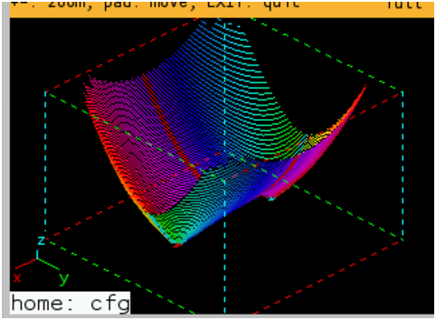
like so-called 4d graphs of the function
from to in the example below
plot3d(x^2-9) :
This geometry application has two main “views” : the graphic view
and the symbolic view, the symbolic view contains Xcas commands that
build the figure displayed in the graphic view, like this
Once the construction is performed,
one can do computation inside the CAS shell, and prove
some conjectures observed in the graphic view. It is also
possible to define intermediate constructions in a CAS
function with the programming editor, and build some parts
of the figure with the help of this function.
2 The geometry application
2.1 Install
You should install the latest version of CAS on your calculator:
- Numworks N0110
- Casio FXCG50, make sure you install the 2 files from the Khicas50 addin
- TI Nspire CX et CX 2 install the alpha version
2.2 Interface
Keyboard shortcuts and screenshots are for a Casio FXCG50.
For a TI Nspire CX or CX II, replace F6 by doc, F4 by menu, EXE by enter, shift EXE by the newline key (bottom right), EXIT by esc. There is no ALPHA key since the Nspire has an alphabetic keyboard.
On a Numworks, replace F6 by Home, F4 by Toolbox, EXE by OK, EXIT by Back, newline (shift EXE) by EXE. Alphabetic lowercase mode is locked by pressing alpha twice, uppercase by another shift alpha.
Fast menus shortcuts on the Nspire and Numworks are shift-1 to shift-9 and a few other shift+keys
2.2.1 Modes, graphical and symbolic view
Type F6 1 (or SD) to display the list
of additional applications, then EXE then select an existing figure
or create a new 2d or 3d figure. You may also open the
geometry application from an existing graph displayed from the shell
(for example after running plot(sin(x)))
by typing F6 then Save figure.
At startup, you are in graphical view in frame mode. The cursor key will modify the viewpoint (move the frame in 2d, rotate viewpoint in 3d). Press F4 to change mode. Type EXE to switch to symbolic view or back. For example, type F4 3 to enter point mode, move the pointer and press EXE where you want to create a point. Or type F4 5 to enter triangle mode move the pointer to each vertex and press EXE on each vertex. You can move the pointer with the keypad (use shift cursor key for a fast move), or if there is an existing point, type the name (e.g. type ALPHA A to move the pointer to the point A if it has already been defined).
In a 3d figure, objects will be created in the yellow plane. Press 4 or 6 to move this plane. It is recommended to keep a viewpoint with vertical (therefore change viewpoint only with the right and left cursor keys that make a rotation of axis ).
Dynamic geometry howto: switch to pointer mode (F4 2), move near an exising point and select it with EXE, then move the point with the cursor keys, you will see how the whole figure depends on that point, this helps conjectures or illustration of some geometric properties, like the fact that 3 lines of a triangle have a common intersection.
If you type EXIT in the graphical view, it will reset mode to frame mode
if you were not in frame mode, or it will switch to symbolic view if
you were in frame mode. In the symbolic view, you can modifiy existing
commands or create new geometric objects with new commandlines (one line
per object). You can save the construction in text format from F6 menu, note
that the file generated will have a .py extension
despite the fact that
it is not a Python script.
Type EXIT again to leave the geometry application.
When leaving the geometry application, the figure is saved in an Xcas variable that has the same identifier than the filename displayed in the symbolic view. You can erase this Xcas variable if you want to clear the figure.
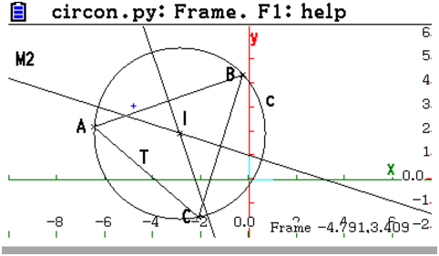
Example : circumcircle.
From KhiCAS shell, type F6 1 then select new figure 2d EXE.
Type F4 5 Triangle, EXE to create the first vertex, move the pointer
with cursor keys and type EXE for the second vertex, move the pointer
again and type EXE to create the 3rd vertex and the triangle.
Long version, construction of the center:
Type F4 7, select 8 Perpen bisector, move the pointer so that
only one edge of the triangle is selected (this is displayed
at the bottom right, something like perpen_bisector D5,D,
type EXE will create the perpendicular bisector. Move the pointer
to another edge of the triangle, type EXE to create the 2nd bisector.
You may optionnaly create the 3rd bisector.
Then type F4 6, select 4 Single intersection. Move the pointer
to a perpen bisector, type EXE, move the pointer to another perpen
bisector and type EXE. This will create the circumcircle center.
Type F4 4, move the pointer to the center (with the cursor keys
or by typing ALPHA H or the center name if it is not H), then EXE,
move to one of the triangle vertex and press EXE.
Short version with the circumcircle command:
Type F4 9, select circumcircle, select each vertex with
pointer move + EXE ((ALPHA A EXE ALPHA B EXE ALPHA C EXE, replace
A, B, C with the vertices names).
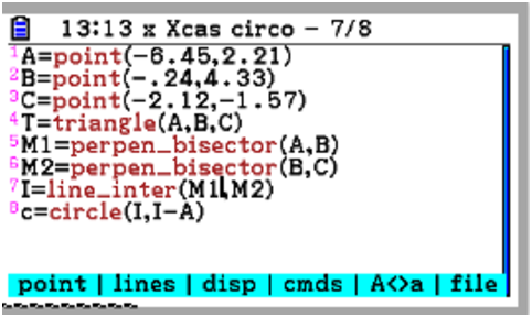
Symbolic view version:
If you are in the graphical view, type EXIT to move to the symbolic view.
Move to the script end and add a newline if required (shift EXE).
Enter
c:=circumcircle(A,B,C) EXE
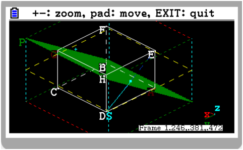
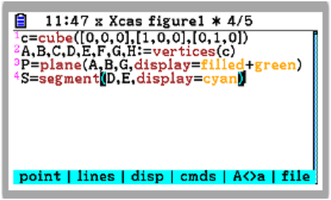
3d Example
c:=cube([0,0,0],[1,0,0],[0,1,0]);
A,B,C,D,E,F,G,H:=vertices(c);
P:=plane(A,B,G,display=filled+green);
S:=segment(D,E,display=cyan);
onload
Type F6 1 from the shell, then select new 3d figure.
Then EXIT or EXE to switch to the symbolic view. Then F5 c ALPHA shift =
F4 uparrow twice, select 3D, EXE 5 for cube, F6 for help on the cube
command, press F2 to copy+paste the first example in the symbolic
view. You should see
c=cube([0,0,0],[1,0,0],[0,1,0])
Type EXE, this display a small cube, type + a few times to zoom in. Then
EXE to switch back to symbolic view.
Type shift EXE to begin a new commandline.
Now we define the vertices of the cube with
A,B,C,D,E,F,G,H=
(type ALPHA A , ALPHA B etc.). Then type F4 and uparrow 3 times
to select Geometry then uparrow 4 times to select
sommets EXE, put c as argument to get sommets(c).
Type EXE to display the cube and the vertices with their names.
Type EXE again to go back to symbolic view. Then shift EXE to
enter a new commandline, that will define the plane ABC.
Type ALPHA P = then F2 to open the fast menu lines and 8, this will
copy plane(.
This command takes 3 points as argument (or a cartesian equation), here
A, B, G, P=plan(A,B,G,. We now add a color to the plane
with the F3 disp fast menu
display=filled+green. Check by EXE EXE.
Go to the next line (shift EXE) and create segment DE
ALPHA S = F2 select segment command with EXE, type D, E, then F3
and give a color
S=segment(D,E,color=cyan)
The whole construction should be
c=cube([0,0,0],[1,0,0],[0,1,0])
A,B,C,D,E,F,G,H=vertices(c)
P=plane(A,B,G,display=filled+green)
S=segment(D,E,display=cyan)
Type EXE to display it and use the keypad to change the viewpoint.
Type EXE or EXIT to go back to symbolic view and EXIT to leave the
geometry application. Type F1 to save the figure if you did not
save it from the F6 menu.
You can access analytic geometry information from KhiCAS shell, for
example equation(P) (F4 select Geometry submenu) will
return the cartesian equation of the plane , or
is_orthogonal(P,S) (F4 Geometry)
will confirm that the plane
is orthogonal to the segment (this should be apparent from
3d rendering).
2.2.2 Cursors
Cursors are parametric values that live in a given inteval and may be
moved by 1% steps from the graphical view. They are created
with the element command in the symbolic view or from F4
menu in the graphical view.
Example : quadratic explorer
This example demonstrates how the curve of the parabola of equation
depends on the value of .
Create 3 cursors from F4 menu of the graphical view
(for each cursor F4 uparrow 4 times EXE EXE). In the symbolic view
you should have something like
a:=element(-1..1)
b:=element(0..1,0.5)
c:=element(-1..1)
then add the parabole graph, from graphical view, type F4 0 (for 10 Curves)
and select plot, or from the symbolic view shift EXE shift F6 and select plot
fill inside the parenthesis with a*x^2+b*x+c (beware,
do not forget the *), then EXE.
From the graphical view, you should see 3 cursors
a, b and c and the corresponding graph.
You can now modify the value of and see how it affects the shape
of the parabola. Type F4 2 (pointer mode), then F5 a (or b or c) EXE
to select (or ( or ). Type EXE then the right and left arrow keys,
EXE again to stop moving the cursor.
A lot of variations may be done, some of them simpler with one or two cursors
and a curve depending on one or two parameters. For example a line equation
explorer with line(y=a*x+b) or a trigonometic explorer with
plot(sin(a*x+b)).
2.2.3 Measures and legends
From the graphical view, type F4 and select 13 Measure. You can compute and display a measure at some point of the figure. For example after creating a triangle, one can display the perimeter of the triangle or its area. Type F4 then uparrow twice EXE. Move the pointer near the triangle, type EXE, move the pointer where you want to display the measure and type EXE.
From the symbolic view, you can display a legend with the
legende() command.
The first argyment of legend may be a point of the figure, or
a vector of 2 integers giving the absolute position in pixels
(measured from the top left corner). The second argument
is the legend, it may be a string or any expression.
If the legend is a numeric value, it can be used as a numeric parameter
for commands that require such an argument, like transformations
(angle of rotation, homothety ratio...)
r:=legend([20,40],"2")
homothety(A,extract_measure(r),B)
2.2.4 Traces
The trace() command lets you keep track of all the positions of
a geometric object when the figure is recomputed while moving a point
Example Enveloppe of the normals to a parametric curve (here an ellipse)
E:=plotparam([cos(t),2*sin(t)],t=-pi..pi)
a:=element(-pi..pi)
M:=element(E,a)
T:=tangent(M)
N:=perpendicular(M,T)
trace(N)
If you change the value of (F4 2 for pointer mode, F5 a),
you will see a curve that separates the area of normals to the curve
and a free area, this is the enveloppe of normals, it is also
the evolute of the ellipse
evolute(E,color=red)
You can remove the traces in the graphical view from the F6 menu (last item).
l:=[];
onload
Click on + several times to see the envelop:
Trace of a point may be useful to conjecture a geometric locus. For example, let and be two points and the circle of diameter . Let be the center of this cercle and a point moving on this circle. Let be the intersection of the tangent to at with the parallel to through . Find the locus of
A:=point(0);
B:=point(1,2);
c:=circle(A,B);
O:=midpoint(A,B);
C:=element(c);
T:=tangent(C);
D2:=parallel(O,droite(A,C));
N:=line_inter(T,D2);
onload
Add the trace(N) command, move in pointer mode and observe
the locus.
2.3 Example mixing geometry and curves
Let and be the curves of the exponential function and its inverse, let and be the tangents to the curves at the points sharing the same abscissa. What are their properties?
Let’s translate this to the calculator, with a cursor that will be the common abscissa:
G=plot(exp(x))
H=plot(exp(-x))
assume(a=1)
M=element(G,a)
N=element(H,a)
T=tangent(M)
U=tangent(N)
simplify(slope(T)*slope(U))There is another property for the intersection of the tangents with the axis:
Ox=line(y=0)
P=line_inter(Ox,T)
Q=line_inter(Ox,U)
Exercice: find this property and prove it with the CAS.
Hints: run the distance command. If you want
to display a result on the figure, run the
legend command.
2.4 Interaction with Xcas
Figures may be saved in text format. They can be copy-pasted to
a geometry level inside Xcas (click on a level number inside
a figure and paste with the ctrl-v shortcut). Conversely, an Xcas
figure level can be saved in text format to a .cas file.
Rename it to a .py extension, transfert it to the calculator,
then it can be inserted inside the symbolic view of a figure.
Recent version of Xcas (1.19-21 at least) can export a session with a geometry level to a CAS session compatible with your calculator without having to copy-paste in text format.
3 Geometry and computer science
Geometry may be used to introduce the algorithmic function concept (that is a procedure that takes arguments and has a return value) in a natural and concrete way (the arguments and return value are geometric objects that we see on the figure).
For example the construction of a circumcircle may be easily
translated to a function taking as arguments the three vertices
of the triangle and returning the center of the circumcircle
(or the circumcircle itself). Just add the function definition header
def f(A,B,C):
and a line to return the center (return I if is
the center), and indent Python-like
def f(A,B,C):
  M1=perpen_bisector(A,B)
  M2=perpen_bisector(B,C)
  I=line_inter(M1,M2)
  return I
Enter this definition (in Xcas syntax, Python-compatible)
inside the programing editor of CAS,
press EXE. Now one can use it inside the geometry application.
It is also possible to define the function directly in the
geometry app editor, but it must be shrinked as a one-liner
and that’s less easily readable
def f(A,B,C): return line_inter(perpen_bisector(A,B),perpen_bisector(B,C))
Exercice : do the same for a sphere circum a tetrahedron
Solution :
def f(A,B,C,D):
  M1=perpen_bisector(A,B)
  M2=perpen_bisector(B,C)
  M3=perpen_bisector(C,D)
  d=line_inter(M1,M2)
  I=line_inter(d,M3)
  return I

A=point(1,2,3)
B=point(2,0,0)
C=point(0,0,-1)
D=point(1,1,-1)
I=f(A,B,C,D)
r=distance(A,I)
tetrahedron(A,B,C,D)
sphere(I,r,display=red)
onload
4 CAS and proof in geometry
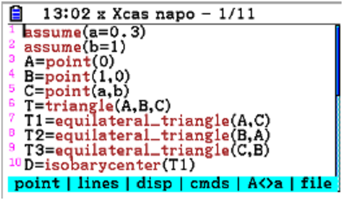
Since the computing kernel is a CAS, it is possible to perform analytic geometry proof with this application. To do that, one should give symbolic values to cursors, if there are enough cursors to be in a generic setting, this gives an analytic geometry proof. For example, in a triangle, one can reduce by translation, rotation and homothety to the case where one vertex is at the origin, the second is and the third depends on two parameters.
assume(a=0.3)
assume(b=1)
A=point(0)
B=point(1)
C=point(a,b)
T=triangle(A,B,C)
The assume command will create a symbolic cursor. It means
that all exact computations will be done with the symbolic value
(e.g. ), while approx computations, e.g. for a graphic
representation, will replace by its numeric value (0.3 here).
This allows viewing a figure (even in a dynamic settings
where and value change)
while keeping analytic computation exact (and unchanged).
After that, one can performe any construction on the triangle. Let’s start with a simple example, show that the three median lines are intersecting at one point, the gravity center of the triangle (also called isobarycenter)
d1=median(A,B,C)
d2=median(B,C,A)
d3=median(C,A,B)
I=line_inter(d1,d2)
This will compute the intersection of two median lines,
then we check that belongs to from a shell command
is_element(I,d3)
The computations were done symbolically, this can be checked
by computing the cartesian equation of
eq:=equation(d3)
Answer: ,
Then we compute the coordinates of
ic:=coordinates(I)
Answer:
We substitute
simplify(subst(eq,[x,y],ic))
Answer: .
By the way, we also get an additional
property of the gravity center of the triangle.
The same can be performed for perpendicular bissectors. For bissectors, computation are much harder and slower, not adapted to a calculator.
Let’s show another theorem with the same setting, Napoleon’s theorem.
Construct three equilateral triangles on each edge of the triangle.
Then the centers of these equilateral triangles are themselve
an equilateral triangle.
On peut faire de même pour les médiatrices. Pour les bissectrices,
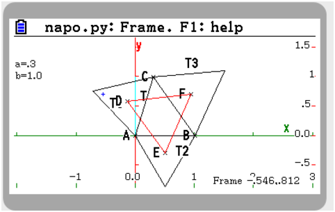
T1:=equilateral_triangle(A,C)
T2:=equilateral_triangle(B,A)
T3:=equilateral_triangle(C,B)
D:=isobarycenter(T1)
E:=isobarycenter(T2)
F:=isobarycenter(T3)
triangle(D,E,F,display=red)
Now let’s prove the theorem, run the following commands in the shell
simplify(distance2(D,E))
simplify(distance2(E,F))
simplify(distance2(F,D))
or with a single command
simplify(distance2(D,E)-distance2(E,F))
Discussion
It must be understood by students that a proof like this is
a full rigorous proof from a mathematical point of view.
It’s not the same as a conjecture that is observed with
a traditional dynamic geometry software with approx data.
Note also that the student has full control on which computations
must be performed, not the software. The software is only
there to perform technical complicated computations.
However, this should not replace a proof obtained by purely geometric arguments, because a geometric proof will force the student work with other interesting concepts. And of course, if an analytic geometry proof can be done by hand, it’s also important that a student learns how to do it without the help of a software.
5 Further reading
If you read French, there are a lot of examples in this manual by Renée De Graeve.
There are links between CAS and geometry in both direction:
- Using CAS to prove geometric results, more precisely a tool named Groebner basis. See for example cet article de D. Kapur
- Geometric theorems may be used to check a CAS kernel. This is the case for Giac/Xcas, classical theorems for median lines, perpendicular bissectors, bissectors and Morley, Feuerbach and Simson theorem are included inside the regression tests basis.