21.4.9  Hilbert-Huang transform

The hht command finds Hilbert spectra by applying the Hilbert-Huang transform (HHT) which obtains instantaneous frequency data from intrinsic mode functions (IMFs) extracted from nonstationary and/or nonlinear signal data. The Hilbert spectrum of a signal reveals its time-dependent features.

• hht takes one mandatory argument and a sequence of optional arguments:
  • data, a list of real numbers (representing the signal) or a matrix in which each row corresponds to an IMF as obtained by empirical mode decomposition (see Section 21.4.8).
  • Optionally, opts, a sequence of optional arguments each of which is one of:
    • frequencies=frng, where frng is either a list [fmin,fmax] or an interval fmin..fmax, where fmin and fmax specify the desired frequency range. The values are in Hertz if sample-rate is provided, otherwise in radians per sample. If frng is a list, then fmin and fmax can also be strings specifying MIDI notes such as e.g. "C4" and "D#5". By default, fmin corresponds to the zero frequency and fmax to the Nyquist frequency.
    • range=trng, where trng is either a list [tmin,tmax] or an interval tmin..tmax, where tmin and tmax specify the desired time range. If sample-rate is provided, then the unit is one second, otherwise the unit is one sample. By default, the entire signal is analyzed.
    • samplerate=sr, where sr is a positive integer representing the sample-rate of the (decomposed) signal (by default, unset).
    • output=out, where out is one of:
      • image (the default), which displays the spectrum as an image.
      • plot, which draws the spectrum with Xcas graphic commands (in lower resolution).
      • matrix, which outputs the spectrum as a matrix in which rows correspond to frequency bins and columns to spectra at individual samples.
    • bins=m, where m is a positive integer specifying the desired number of bins for the frequency range discretization. By default, m=200 for the image output and m=100 for the plot and matrix outputs.
    • log=islog, where islog is a boolean value specifying whether the frequency axis is logarithmic or not (by default, the scale is linear). If islog=true, then the frequency-axis unit is one semitone, with zero corresponding to the MIDI note 0. Instead of log=true, you can simply enter log.
    • legend=haslegend, where haslegend is a boolean value specifying whether to show the colormap or not (by default, the colormap is shown on the right of the spectrum).
    • tran=hasalpha, where hasalpha is a boolean value specifying whether to use the alpha channel in the image output (this value is ignored for other outputs). When used, the alpha channel values are smaller for smaller amplitudes, making the lower-amplitude components less visible. By default, tran=true.
    • color=cmap, where cmap is the colormap index (nonnegative integer) as returned by the colormap command (see Section 19.1.3). cmap can also be a boolean value, with true corresponding to the default rainbow colormap and false corresponding to the grey ramp with 24 colors from the FLTK colormap. A suitable choice of colormap can help detecting important signal features in the graphic output. By default, color=true.
• hht(data ⟨,opts ⟩) returns (the selected part of) the Hilbert spectrum associated with data in the specified form. If graphic output is selected, then the colormap is used to color-encode amplitude data. The axis units are seconds/samples resp. Hertz/radians per second/semitones, depending on the values of samplerate and log options.
• With matrix output, you can use hht to compute the signal energy as a function of time. The element at position (i,j) in the resulting matrix, when squared, represents the energy of the ith frequency bin at the jth sample. The total energy at time j is the sum of squares of elements in the jth column of the matrix.

Examples

Synthetic signal.

To see the spectrum of the synth signal defined in Section 21.4.8 with the FLTK grayscale ramp, enter:

You may also pass the list of already computed IMFs as the first argument.

Whale song.

The file nepblue24s10x.wav downloaded from here contains sounds produced by a blue whale in the northeast Pacific. Since the frequency of moans is very low (below 20 Hz, which is inaudible for humans), the file is played back at 10x speed. To load and show the audio, enter:

You can hear the whale song by entering (see Section 28.2.14):

To perform the empirical mode decomposition (see Section 21.4.8), enter:

Evaluation time: 10.01

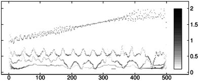
(Note that the residue is discarded since it is not relevant for the spectrum.) To display the Hilbert spectrum of the whale song, enter:

Whale moans occur at about 5, 10, 15 and 20 seconds from the beginning of the recording (in reality, these intervals are ten times larger). Also, the spectrum reveals that moans have the same frequency, about 160 Hz in the recording and 16 Hz in reality. The magnitude of the first moan is smaller, as suggested by both the waveform and spectrum.

To obtain the Hilbert spectrum as a matrix, enter:

To plot the energy of the whale song, sum the columns of the Hilbert spectrum matrix in which every element is squared. Energy data can be smoothed out by applying a moving-average filter.

Spectral analysis of music.

With the file CantinaBand3.wav downloaded from here:

To obtain instrinsic mode functions, enter (residue is discarded):

To display the Hilbert spectrum of music, enter:

In the upper part of the spectrum you can see individual beats of the song, and in the lower part you can see six bass notes appearing every 2 beats. The first and fifth notes are stressed more than the others, suggesting the 4/4 time signature. The percussive pickup measure is also clearly visible. The first beat of the first measure starts after about 0.65 seconds. In the example in Section 21.4.5 it is explained how to extract the rhythmic section by cutting out the middle band of the spectrum.

As another example, download the files violin-C4.wav and flute-G6.wav from here and load them:

Mix the two audio clips with one-second delay for the flute (see Section 28.2.18):

You can hear the result by using the playsnd command (see Section 28.2.14). To display the Hilbert spectrum, enter (in this case, EMD is computed automatically by hht):

The specified colormap helps you to see two individual tones at 60 resp. 91 semitones from the MIDI note 0, corresponding to C4 resp. G6, as expected. The flute part of the spectrum (yellow-reddish) is much more concentrated than the violin part due to the inherent sinusoidal quality of the flute sound.