20.4.22 Kernel density estimation
The kernel_density
or kde
command performs kernel density estimation
(KDE)1.
kernel_density takes a sample, optionally
restricted to an interval [a,b], and obtains an estimate f of
the (unknown) probability density function f from which the samples
are drawn. The function f is defined by:
|
f(x)= | | | | K | ⎛
⎜
⎜
⎝ | | ⎞
⎟
⎟
⎠ | ,
(13) |
where K is the Gaussian kernel
| K(u)= | | exp | ⎛
⎜
⎜
⎝ | − | | u2 | ⎞
⎟
⎟
⎠ |
and h is the positive real parameter called the bandwidth.
-
kernel_density takes one mandatory argument and a
sequence of optional arguments:
-
L, a list of samples L=[X1,X2,…,Xn].
- Optionally, a sequence of options from:
-
output=type (or
Output=type to specify the form of the return
value f, where type can be one of:
-
exact, to return f as the sum of
Gaussian kernels, i.e. as the right side of (13),
which is usable only when the number of samples is relatively
small (up to few hundreds).
- piecewise, to return f as a piecewise
expression obtained by the spline interpolation of the
specified degree (by default, the interpolation is linear) on
the interval [a,b] segmented to the specified number of bins.
- list (the default), to return f in
discrete form, as a list of values
f(a+k b−a/M−1) for
k=0,1,…,M, where M is the number of bins.
-
bandwidth=value, to specify the bandwidth.
value can be one of:
-
h, a positive real number.
- select (the default), to have the bandwidth
selected using a direct plug-in method,
- gauss (or normal or normald)
to use Silverman’s rule of thumb for selecting
bandwidth (this method is fast but the results are close to
optimal ones only when f is approximately normal).
-
bins=n for a positive integer n (by default
100), the number of bins for simplifying the input data. Only the
number if samples in each bin is stored. Bins represent the
elements of an equidistant segmentation of the interval S on
which KDE is performed. This allows evaluating kernel summations
using convolution when output is set to
piecewise or list, which significantly lowers
the computational burden for large values of n (say, few
hundreds or more). If output is set to exact,
this option is ignored.
- a..b or range=[a,b] or
x=a..b for real numbers a and b, to specify the
interval [a,b] on which KDE is performed. If an identifier x
is specified, it is used as the variable of the output. If the
range endpoints are not specified, they are set to a=min1≤
i≤ n Xi−3 h and b=max1≤ i≤ nXi+3 h (unless
output is set to exact, in which case this
option is ignored).
- interp=n for an integer n (by default 1), which
specifies the degree of the spline interpolation, ignored unless
output is set to piecewise.
- spline=n for an integer n, which sets
option to piecewise and interp to n.
- eval=x0 to only return the value
f(x0) (this cannot be used with output set to list).
- x, an unassigned identifier (by default x) to use
as the variable of the output.
- exact, the same as output=exact.
- piecewise, the same as output=piecewise.
- kernel_density(L ⟨,options ⟩)
returns the function f given in (13).
Examples
| kernel_density([1,2,3,2],bandwidth=1/4,exact) |
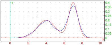
| f:=unapply(normald(4,1,x)/2+normald(7,1/2,x)/2,x) |
| X:=randvar(f,range=0..10,1000):;
S:=sample(X,1000):;
F:=kernel_density(S,piecewise):;
plotfunc([f(x),F],x=0..10,color=[red,blue]) |
The exact density is drawn in red.
| kernel_density(S,bins=50,spline=3,eval=4.75) |
| time(kernel_density(sample(X,1e5),piecewise)) |
| S:=sample(X,5000):;
sqrt(int((f(x)-kde(S,piecewise))^2,x=0..10)) |
| S:=sample(X,25000):;
sqrt(int((f(x)-kde(S,bins=150,piecewise))^2,x=0..10)) |